Finding Adjusted Daily Returns of Stocks with R
- Eda Coşkun

- Sep 2, 2020
- 5 min read
Updated: Sep 23, 2020
You are looking at the Yahoo Finance, monitoring returns of several stocks and think about how can you get the relevant information in this excessive amount of data and make simple but meaningful results from them. Thankfully, R provides you with great tools for manipulating the data for your own interest of use.
In this post, I will download stock data using quantmod and the Yahoo Finance API and manipulate the data using some R sub-setting functions. I will pull down adjusted daily return stock data using Microsoft's and Facebook's stock. Then combine data for comparison. With the combined data, I will practice calculating the Sharp Ratio on multiple stocks to see which stock is truly the riskier asset or the stock with the best risk return profile.
So let's get started
Derive the stock data for Microsoft (MSFT)
MSFT<-getSymbols("MSFT",auto.assign = F) #getSymbols returns stock data for the variables you choose## 'getSymbols' currently uses auto.assign=TRUE by default, but will
## use auto.assign=FALSE in 0.5-0. You will still be able to use
## 'loadSymbols' to automatically load data. getOption("getSymbols.env")
## and getOption("getSymbols.auto.assign") will still be checked for
## alternate defaults.
##
## This message is shown once per session and may be disabled by setting
## options("getSymbols.warning4.0"=FALSE). See ?getSymbols for details.head(MSFT)#visualize first 5 rows of data set## MSFT.Open MSFT.High MSFT.Low MSFT.Close MSFT.Volume MSFT.Adjusted
## 2007-01-03 29.91 30.25 29.40 29.86 76935100 22.07034
## 2007-01-04 29.70 29.97 29.44 29.81 45774500 22.03338
## 2007-01-05 29.63 29.75 29.45 29.64 44607200 21.90772
## 2007-01-08 29.65 30.10 29.53 29.93 50220200 22.12207
## 2007-01-09 30.00 30.18 29.73 29.96 44636600 22.14425
## 2007-01-10 29.80 29.89 29.43 29.66 55017400 21.92251tail(MSFT)#visualize last 5 rows of data set## MSFT.Open MSFT.High MSFT.Low MSFT.Close MSFT.Volume MSFT.Adjusted
## 2020-08-25 213.10 216.61 213.10 216.47 23043700 216.47
## 2020-08-26 217.88 222.09 217.36 221.15 39600800 221.15
## 2020-08-27 222.89 231.15 219.40 226.58 57602200 226.58
## 2020-08-28 228.18 230.64 226.58 228.91 26292900 228.91
## 2020-08-31 227.00 228.70 224.31 225.53 28774200 225.53
## 2020-09-01 225.51 227.45 224.43 227.27 25725500 227.27df_MSFT<- as.data.frame(MSFT)
class(MSFT) #check whether we can store the msft as data frame## [1] "xts" "zoo"class(df_MSFT)## [1] "data.frame"Derive the stock data for Amazon
AMZN<-getSymbols("AMZN",auto.assign = F)
df_AMZN<- as.data.frame(AMZN)  #store as data frame

str(df_AMZN) #str() allows the user to see what type of object the data frame is.
## 'data.frame': 3441 obs. of 6 variables:
## $ AMZN.Open : num 38.7 38.6 38.7 38.2 37.6 ...
## $ AMZN.High : num 39.1 39.1 38.8 38.3 38.1 ...
## $ AMZN.Low : num 38 38.3 37.6 37.2 37.3 ...
## $ AMZN.Close : num 38.7 38.9 38.4 37.5 37.8 ...
## $ AMZN.Volume : num 12405100 6318400 6619700 6783000 5703000 ...
## $ AMZN.Adjusted: num 38.7 38.9 38.4 37.5 37.8 ...summary(df_AMZN)# statistical summary of numerical variables## AMZN.Open AMZN.High AMZN.Low AMZN.Close
## Min. : 35.29 Min. : 37.07 Min. : 34.68 Min. : 35.03
## 1st Qu.: 131.05 1st Qu.: 132.80 1st Qu.: 129.53 1st Qu.: 131.31
## Median : 303.91 Median : 306.21 Median : 300.17 Median : 303.83
## Mean : 630.22 Mean : 637.00 Mean : 622.86 Mean : 630.34
## 3rd Qu.: 887.50 3rd Qu.: 893.49 3rd Qu.: 884.49 3rd Qu.: 886.54
## Max. :3489.58 Max. :3513.87 Max. :3467.00 Max. :3499.12
## AMZN.Volume AMZN.Adjusted
## Min. : 881300 Min. : 35.03
## 1st Qu.: 3086500 1st Qu.: 131.31
## Median : 4495100 Median : 303.83
## Mean : 5625767 Mean : 630.34
## 3rd Qu.: 6769300 3rd Qu.: 886.54
## Max. :104329200 Max. :3499.12head(df_AMZN)## AMZN.Open AMZN.High AMZN.Low AMZN.Close AMZN.Volume AMZN.Adjusted
## 2007-01-03 38.68 39.06 38.05 38.70 12405100 38.70
## 2007-01-04 38.59 39.14 38.26 38.90 6318400 38.90
## 2007-01-05 38.72 38.79 37.60 38.37 6619700 38.37
## 2007-01-08 38.22 38.31 37.17 37.50 6783000 37.50
## 2007-01-09 37.60 38.06 37.34 37.78 5703000 37.78
## 2007-01-10 37.49 37.70 37.07 37.15 6527500 37.15Store the data frame in csv format
write.csv(df_AMZN,file = "amzn stock") Find the daily return of the adjusted closing stock price
daily_msft<-dailyReturn(MSFT$MSFT.Adjusted)
head(daily_msft)
## daily.returns
## 2007-01-03 0.000000000
## 2007-01-04 -0.001674736
## 2007-01-05 -0.005703029
## 2007-01-08 0.009784129
## 2007-01-09 0.001002664
## 2007-01-10 -0.010013388Visualize the first 10 row (head) the monthly return of the adjusted closing stock price and store as monthly_msft
head(monthlyReturn(MSFT$MSFT.Adjusted),10)## monthly.returns
## 2007-01-31 0.033489058
## 2007-02-28 -0.084002434
## 2007-03-30 -0.010649770
## 2007-04-30 0.074273600
## 2007-05-31 0.028370680
## 2007-06-29 -0.039752314
## 2007-07-31 -0.016287909
## 2007-08-31 -0.005495093
## 2007-09-28 0.025409005
## 2007-10-31 0.249491301monthly_msft<-monthlyReturn(MSFT$MSFT.Adjusted)Visualize the first 10 row (head) the yearly return of the adjusted closing stock price and store as yearly_msft
head(yearlyReturn(MSFT$MSFT.Adjusted),10)## yearly.returns
## 2007-12-31 0.20842884
## 2008-12-31 -0.44385606
## 2009-12-31 0.60467155
## 2010-12-31 -0.06524647
## 2011-12-30 -0.04515672
## 2012-12-31 0.05798857
## 2013-12-31 0.44297966
## 2014-12-31 0.27564613
## 2015-12-31 0.22691902
## 2016-12-30 0.15077722yearly_msft<-yearlyReturn(MSFT$MSFT.Adjusted)Plot the daily returns
plot(daily_msft,type = 1)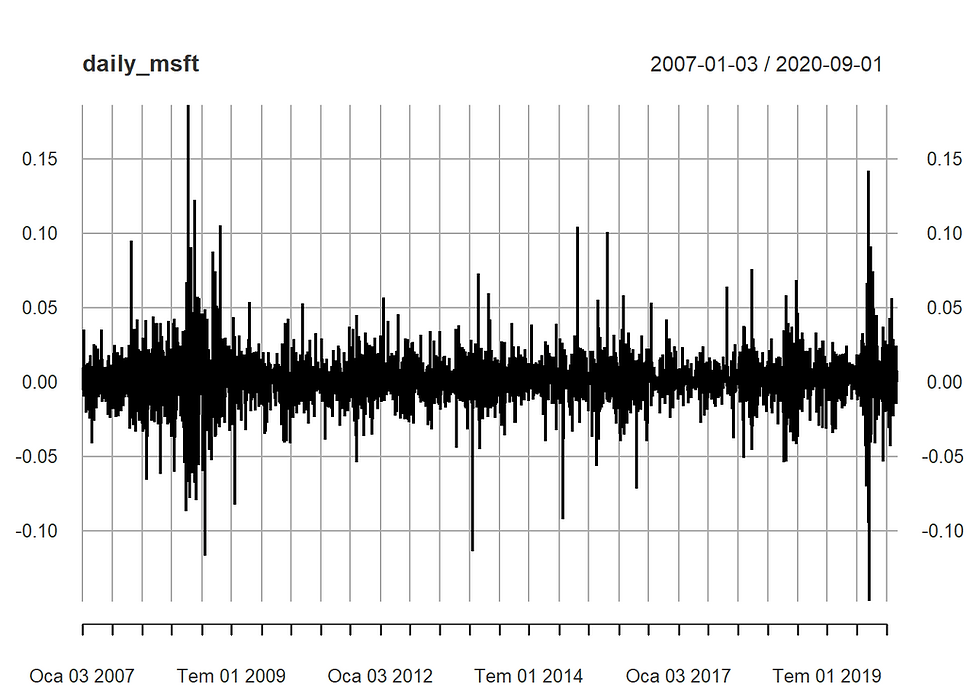
Adjusted returns step by step
msft_adj<- Ad(MSFT)#take only adjusted returns
msft_adj_daily<-dailyReturn(msft_adj)#store the daily adjusted returns
head(msft_adj_daily)
## daily.returns
## 2007-01-03 0.000000000
## 2007-01-04 -0.001674736
## 2007-01-05 -0.005703029
## 2007-01-08 0.009784129
## 2007-01-09 0.001002664
## 2007-01-10 -0.010013388head(daily_msft)#msft_adj_daily and daily_msft are equivalent## daily.returns
## 2007-01-03 0.000000000
## 2007-01-04 -0.001674736
## 2007-01-05 -0.005703029
## 2007-01-08 0.009784129
## 2007-01-09 0.001002664
## 2007-01-10 -0.010013388Finding daily adjusted returns in only one step
new_msft<-dailyReturn(Ad(getSymbols("MSFT",auto.assign = F)))
head(new_msft)
## daily.returns
## 2007-01-03 0.000000000
## 2007-01-04 -0.001674736
## 2007-01-05 -0.005703029
## 2007-01-08 0.009784129
## 2007-01-09 0.001002664
## 2007-01-10 -0.010013388Finding the daily return of adjusted closing stock price for Facebook
fb<- getSymbols("FB",auto.assign = F)
fb_ad<- Ad(fb)
fb_daily<- dailyReturn(fb_ad)
head(fb_daily)
## daily.returns
## 2012-05-18 0.00000000
## 2012-05-21 -0.10986139
## 2012-05-22 -0.08903906
## 2012-05-23 0.03225806
## 2012-05-24 0.03218747
## 2012-05-25 -0.03390854Finding fb_daily in shorter way
new_fb<-dailyReturn(Ad(getSymbols("FB",auto.assign = F)))Joining two stocks data sets into one data set
comb_traded<-merge(new_msft,new_fb,all=F)Rename the column names for better visualization
colnames(comb_traded)## [1] "daily.returns" "daily.returns.1"names(comb_traded)[names(comb_traded) == "daily.returns"] <- "MSFT.returns"
names(comb_traded)[names(comb_traded) == "daily.returns.1"] <- "FB.returns"Compare the daily returns of Facebook with Microsoft
charts.PerformanceSummary(comb_traded,main="FB-Microsoft")
Annualized Returns and Sharp Ratio
Note! The risk-free rate of return means theoretical rate of return of an investment with zero risk, however, in practice every investment carries at least small amount of risk.
To solve this issue we find an approximate risk-free rate of return, while considering investor’s home market. For example, for U.S. based investors the interest rate on a three-month U.S. Treasury bill is often used as the risk-free rate.
table.AnnualizedReturns(comb_traded,scale = 252,Rf= .004/252)#RF is risk-free rate## MSFT.returns FB.returns
## Annualized Return 0.3079 0.2802
## Annualized Std Dev 0.2595 0.3741
## Annualized Sharpe (Rf=0.4%) 1.1661 0.7353Std dev is standard deviation which is a measure of dispersion relative to its mean. It is the square root of variance (volatility)
Sharp ratio is the average return earned in excess of the risk-free rate per unit of volatility or total risk
Generally, the greater the value of the Sharpe ratio, the more attractive the risk-adjusted return.
So as a result, it is shown that Microsoft has higher sharpe ratio which makes it more attractive than Facebook’s stocks
If you want to see this project's R markdown file or find relevant projects, you can go to RPubs and visit edacoskun
The link for this project is
https://rpubs.com/edacoskun/655251


Comments